Recently I found this helpful course to help me learn how to actually start writing some Neural Networks. I understand the theory fairly well, but I wanted to actually write one and play around with it. This course showcases a data science competition website called Kaggle that provides a ton of datasets, helpful discussions, and the ability to write/fork some Jupyter notebooks directly on the site. Kaggle provides some tutorial competitions, the first one being a competition to predict who lived and died on the titanic. This is a pretty straight forward problem, and it has a ton of discussion topics and Kernels to get started. You can even check out my notebook getting a 0.76 score in the competition and play around with the code in this article. This problem isn’t super well suited for Nerual Networks, but I thought I would try anyways.
To follow along with this tutorial, make sure to install keras and if you want to get fancy, install jupyter, it is a pretty nice tool for playing around with data science. Finally, download the competition training and test data.
Setup some potential models
I have no idea what form of model I should use, so I’m making some methods that use various architectures to see if any of them give better performance. After experminenting with these approaches, I found that the simple model performs the best. Feel free to play around with the other models to see if you can make any of them better. These examples are pretty much pulled directly from the Keras documentation which provides some helpful information on what this code means.
from keras.models import Sequential
from keras.layers import Dense, Activation, Dropout

# Simpel model that only has one Dense input layer and one output layer.
def create_model_simple(input_size):
    model = Sequential([
        Dense(512, input_dim=input_size),
        Activation('relu'),
        Dense(1),
        Activation('sigmoid'),
    ])

    # For a binary classification problem
    model.compile(optimizer='adam',
              loss='binary_crossentropy',
              metrics=['accuracy'])

    return model

# Slightly more complex model with 1 hidden layer
def create_model_multiple_layers(input_size):
    model = Sequential([
        Dense(512, input_dim=input_size),
        Activation('relu'),
        Dense(128),
        Activation('relu'),
        Dense(1),
        Activation('sigmoid'),
    ])

    # For a binary classification problem
    model.compile(optimizer='adam',
              loss='binary_crossentropy',
              metrics=['accuracy'])

    return model

# Simple model with a dropout layer thrown in
def create_model_dropout(input_size):
    model = Sequential([
        Dense(512, input_dim=input_size),
        Activation('relu'),
        Dropout(0.1),
        Dense(1),
        Activation('sigmoid'),
    ])

    # For a binary classification problem
    model.compile(optimizer='adam',
              loss='binary_crossentropy',
              metrics=['accuracy'])

    return model

# Slightly more complex model with 2 hidden layers and a dropout layer
def create_model_complex(input_size):
    model = Sequential([
        Dense(512, input_dim=input_size),
        Activation('relu'),
        Dropout(0.2),
        Dense(128),
        Activation('relu'),
        Dropout(0.2),
        Dense(1),
        Activation('sigmoid'),
    ])

    # For a binary classification problem
    model.compile(optimizer='adam',
              loss='binary_crossentropy',
              metrics=['accuracy'])

    return model
Now that we can create our models, let’s make one with an arbitrary input size and summarize it with Keras.
summarize_model = create_model_simple(10)
model.summary()
____________________________________________________________________________________________________
Layer (type)                     Output Shape          Param #     Connected to
====================================================================================================
dense_5 (Dense)                  (None, 512)           3072        dense_input_3[0][0]
____________________________________________________________________________________________________
activation_5 (Activation)        (None, 512)           0           dense_5[0][0]
____________________________________________________________________________________________________
dense_6 (Dense)                  (None, 1)             513         activation_5[0][0]
____________________________________________________________________________________________________
activation_6 (Activation)        (None, 1)             0           dense_6[0][0]
====================================================================================================
Total params: 3,585
Trainable params: 3,585
Non-trainable params: 0
____________________________________________________________________________________________________
Format the data
Now that we have a basic model setup we have to do the hard part: data cleanup. I’m using some tips found in this helpful kernel to make sure I don’t have misleading data that will confuse the model. For example, the Cabin data is so sparse (filled with NaN values) that data will most likely just cause problems for our model. In order for us to get a better idea of how our model will handle unknown data, I’m going to extract a subset of training data to set aside for testing (it will not be included in the training set, but it will be used to see how well our model predicts).
def format_data(dataframe):
# drop unnecessary columns
# PassengerId is always different for each passenger, not helpful
# Name is different for each passenger, not helpful (maybe last names would be helpful?)
# Ticket information is different for each passenger, not helpful
# Embarked does not have any strong correlation for survival rate.
# Cabin data is very sparse, not helpful
dataframe = dataframe.drop(['PassengerId','Name','Ticket','Embarked','Cabin'], axis=1)
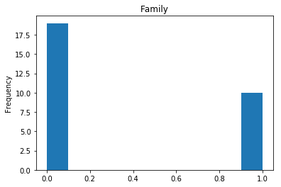
# Instead of having two columns Parch & SibSp,
# we can have only one column represent if the passenger had any family member aboard or not,
# Meaning, if having any family member(whether parent, brother, ...etc) will increase chances of Survival or not.
dataframe['Family'] = dataframe["Parch"] + dataframe["SibSp"]
dataframe['Family'].loc[dataframe['Family'] > 0] = 1
dataframe['Family'].loc[dataframe['Family'] == 0] = 0
# drop Parch & SibSp
dataframe = dataframe.drop(['SibSp','Parch'], axis=1)
# get average, std, and number of NaN values in titanic_df
average_age_titanic = dataframe["Age"].mean()
std_age_titanic = dataframe["Age"].std()
count_nan_age_titanic = dataframe["Age"].isnull().sum()
# generate random numbers between (mean - std) & (mean + std)
rand_1 = np.random.randint(average_age_titanic - std_age_titanic, average_age_titanic + std_age_titanic,
size = count_nan_age_titanic)
dataframe["Age"][np.isnan(dataframe["Age"])] = rand_1
return dataframe
def string_to_numbers(data, dataframe, encoder):
# assign labels for all the non-numeric fields
headings = list(dataframe.columns.values)
for heading_index in range(len(headings)):
dataframe_type = dataframe[headings[heading_index]].dtype
column = data[:,heading_index]
if dataframe_type == np.int64 or dataframe_type == np.float64:
data[:,heading_index] = column.astype(float)
else :
data[:,heading_index] = encoder.fit(column).transform(column).astype(float)
return data
import pandas
import numpy as np
import sklearn.preprocessing as preprocessing

from sklearn.preprocessing import LabelEncoder

# load dataset
titanic_df = pandas.read_csv('data/titanic/train.csv')
# format the data
titanic_df = format_data(titanic_df)

# pull out the correct answers (survived or not)
Y_train = titanic_df["Survived"].values

# drop the survived column for the training data
titanic_df = titanic_df.drop("Survived",axis=1)

X_train = titanic_df.values

# assign labels for all the non-numeric fields
encoder = LabelEncoder()
X_train = string_to_numbers(X_train, titanic_df, encoder)

# Extract a small validation set
validation_set_size = 200
random_indices = np.random.randint(low=0,high=len(X_train)-1,size=validation_set_size)
X_valid = X_train[random_indices]
Y_valid = Y_train[random_indices]
X_train = np.delete(X_train, random_indices, axis=0)
Y_train = np.delete(Y_train, random_indices, axis=0)

# normalize the data
preprocessing.scale(X_train)
preprocessing.scale(X_valid)
Train the model
Here is the heart of neural networks: training. I won’t go over how training works in this article, but this is how we generate the weights our network will use to try and predict who lived and who died in our test data.
from keras.wrappers.scikit_learn import KerasClassifier
from sklearn.model_selection import cross_val_score
from sklearn.model_selection import StratifiedKFold
from sklearn.preprocessing import StandardScaler
from sklearn.pipeline import Pipeline

# Train the model, iterating on the data in batches of 64 samples
model = create_model_simple(len(X_train[0]))

model.optimizer.lr = 0.01
model.fit(X_train, Y_train, nb_epoch=100, batch_size=64)
Epoch 100/100
715/715 [==============================] - 0s - loss: 0.4917 - acc: 0.7706
This output tells us that after 100 epochs, our model was able to accurately predict 77% of the training data. Not great, so lets look at how the model performs when predicting to see if we can make it better.
Visualize Predictions on Validation Set
Now we want to visualize how our model performs. We want to see what kinds of passengers the model is good at guessing, and what it is bad at. In order to visualize this, we are going to have our model predict whether or not the survivors in our validation set (the small subset we pulled out of our training data) lived or died. Since we know the correct answers, we can see how our model performed.
# run predictions on our training data
train_preds = model.predict(X_valid, batch_size=64)
rounded_preds = np.round(train_preds).astype(int).flatten()
correct_preds = np.where(rounded_preds==Y_valid)[0]
print("Accuracy: {}%".format(float(len(correct_preds))/float(len(rounded_preds))*100))
Accuracy: 83.0%
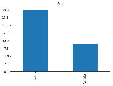
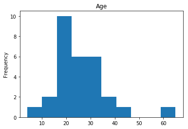
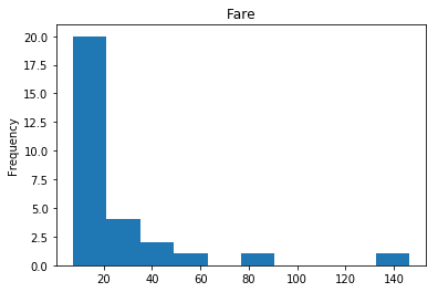
We want to visualize the distributions of the various data provided in the training data to see if we can find any patterns in which passengers the data is good at guessing or not good at guessing. In order to do that, we will setup some methods that can render the numerical and the string data.
import matplotlib.pyplot as plt

def render_value_frequency(dataframe, title):
    fig, ax = plt.subplots()
    dataframe.value_counts().plot(ax=ax, title=title, kind='bar')
    plt.show()

def render_plots(dataframes):
    headings = dataframes.columns.values
    for heading in headings:
        data_type = dataframes[heading].dtype
        if data_type == np.int64 or data_type == np.float64:
            dataframes[heading].plot(kind='hist',title=heading)
            plt.show()
        else:
            render_value_frequency(dataframes[heading],heading)
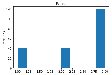
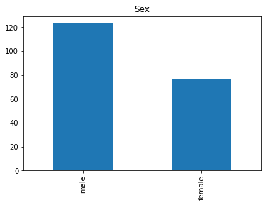
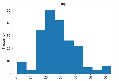
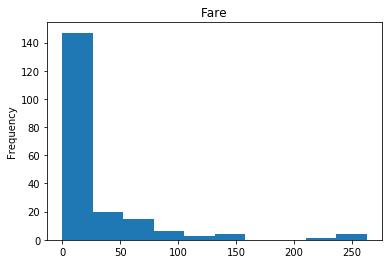
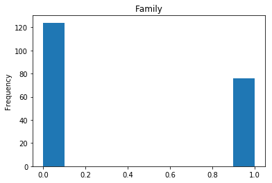
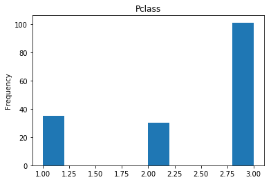
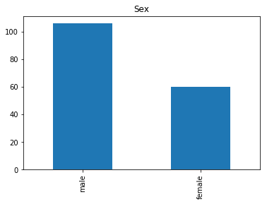
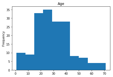
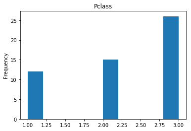
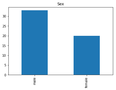
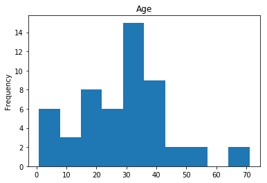
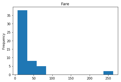
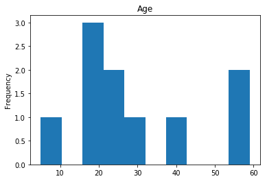
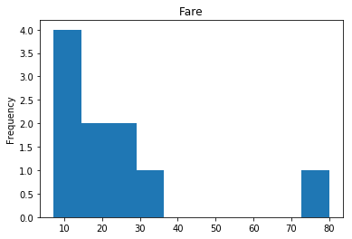
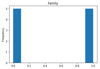
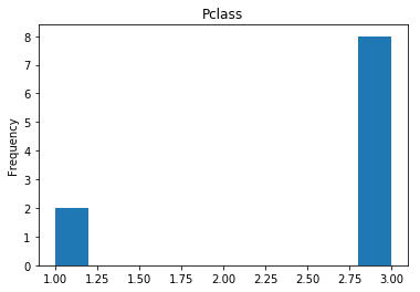
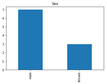
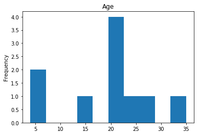
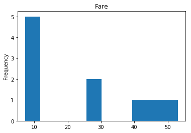
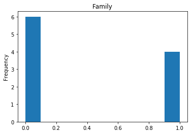
Distributions
First let’s render the plots for all of our data so we can see the general distribution.
render_plots(titanic_df.iloc[random_indices])
Correct
First we will look at what our model is good at. These are all of the correct predictions our model made on our validation set. We are going to plot all of the data we know about the passengers the model got right, and check if we see any patterns.
# find the indices of all of the correct predictions (prediction matches the expected label)
correct = np.where(rounded_preds==Y_valid)[0]
print("Found {} correct labels".format(len(correct)))
render_plots(titanic_df.iloc[correct])
Found 166 correct labels
Incorrect
Next we see what our model is bad at, all of our incorrect guesses.
# find all the indices where the prediction did not match the correct label
incorrect = np.where(rounded_preds!=Y_valid)[0]
print("Found {} incorrect labels".format(len(incorrect)))
render_plots(titanic_df.iloc[incorrect])
Found 11 incorrect labels
Confident Survived and Survived
Now we get into the more interesting data sets. This one is seeing which of our predictions had the highest probability of being correct, and they were correct.
# find all the indices where the prediction label probability was highest
confident_survived_correct = np.where((rounded_preds==1) & (rounded_preds==Y_valid))[0]
print("Found {} confident correct survived labels".format(len(confident_survived_correct)))
render_plots(titanic_df.iloc[confident_survived_correct])
Found 29 confident correct survived labels
Confident Died and Died
Similar to the last operation, we will see the data where the model is confident a passenger died.
# find all the indices where the prediction label probability was the lowest
confident_died_correct = np.where((rounded_preds==0) & (rounded_preds==Y_valid))[0]
print("Found {} confident correct died labels".format(len(confident_died_correct)))
render_plots(titanic_df.iloc[confident_died_correct])
Found 53 confident correct died labels
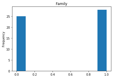
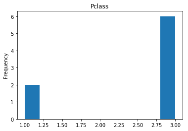
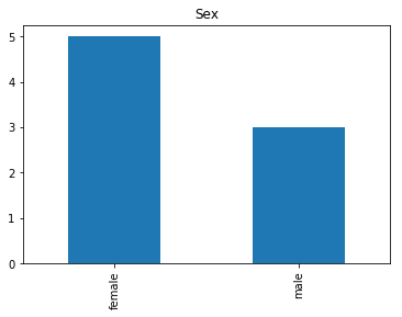
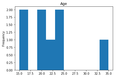
Confident Survived and Died
Now we get into the really interesting stuff. These are the labels where our model was very confident, but was wrong.
# find all the indices where the predicted label probability was high, but incorrect
confident_survived_incorrect = np.where((rounded_preds==1) & (rounded_preds!=Y_valid))[0]
print("Found {} confident incorrect survived labels".format(len(confident_survived_incorrect)))
render_plots(titanic_df.iloc[confident_survived_incorrect])
Found 8 confident incorrect survived labels
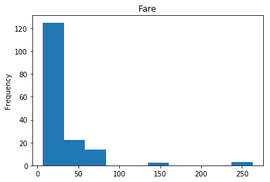
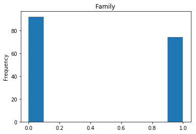
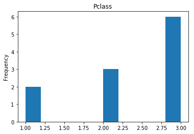
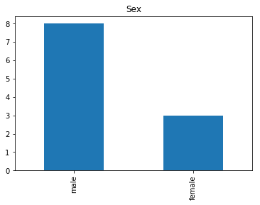
Confident Died and Survived
# find all the indices where the predicted label probability was low, but incorrect
confident_died_incorrect = np.where((rounded_preds==0) & (rounded_preds!=Y_valid))[0]
print("Found {} confident incorrect died labels".format(len(confident_died_incorrect)))
render_plots(titanic_df.iloc[confident_died_incorrect])
Found 10 confident incorrect died labels
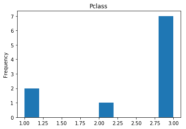
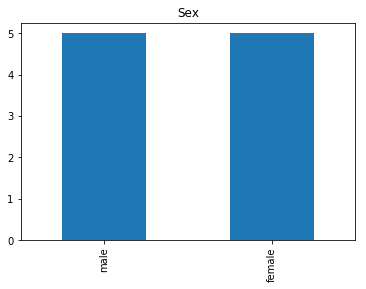
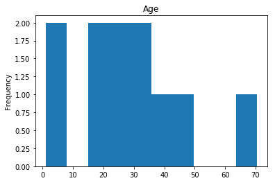
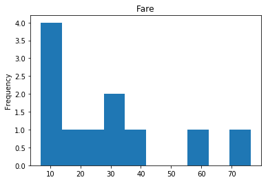
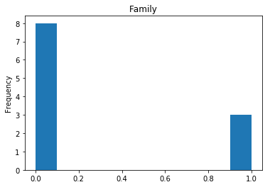
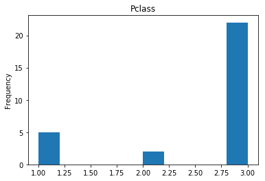
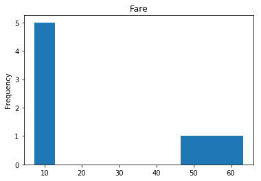
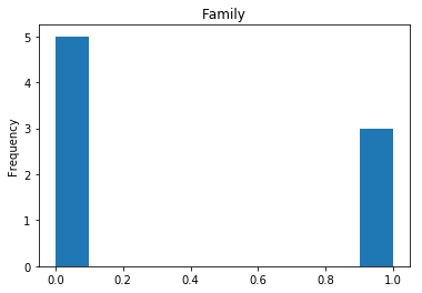
Uncertain
Finally, we see what our model isn’t sure about. These are the 10 most uncertain labels that our model guessed at.
# sort the array indices by the values closest to 0.5
most_uncertain = np.argsort(np.abs(train_preds.flatten()-0.5))[:10]
render_plots(titanic_df.iloc[most_uncertain])
Analyze the Trends
So now we have some visualization on how well our model performs. This would be what I consider the hardest part of data science, and why it seems like nerual networks are super difficult. We have to look at the data, and we have to find the trends so we can make our model better. That may mean dropping data that proves misleading. For example, if we determined that Age really doesn’t play into if someone lived or died (which I would guess is wrong, being a child most certainly should provide a good guess about living or dying) we can drop that data completely and see if our model performs better. I am far from a data scientist, so my guesses at these trends are probably way off but I’ll try anyway.
My best guess is that there are quite a few cases where there are people that statistically were likely to die or survive, but due to the randomness of the scenario defied the expectations. I can’t really see any noticable trends in the data that would suggest the model is treating any data point as more important than it should be. So, I’ll test out my own theory that the most important factor for living or dying is class. So I’m going to train and test the model again after removing what I consider to be the outliers that are confusing the model.
# load dataset
titanic_df_no_outliers = pandas.read_csv('data/titanic/train.csv')
# format the data
titanic_df_no_outliers = format_data(titanic_df_no_outliers)

# attempt to remove all of the "outliers", things like high class female passengers who died (likely to live) or
# low class males surviving (likely to die)
titanic_df_no_outliers = titanic_df_no_outliers.drop(titanic_df_no_outliers[(titanic_df_no_outliers["Pclass"] == 1) & (titanic_df_no_outliers["Age"] >= 10) & (titanic_df_no_outliers["Survived"] == 0)].index)
titanic_df_no_outliers = titanic_df_no_outliers.drop(titanic_df_no_outliers[(titanic_df_no_outliers["Pclass"] == 3) & (titanic_df_no_outliers["Age"] >= 10) & (titanic_df_no_outliers["Survived"] == 1)].index)

# pull out the correct answers (survived or not)
Y_train_no_outliers = titanic_df_no_outliers["Survived"].values

# drop the survived column for the training data
titanic_df_no_outliers = titanic_df_no_outliers.drop("Survived",axis=1)

X_train_no_outliers = titanic_df_no_outliers.values

# assign labels for all the non-numeric fields
encoder = LabelEncoder()
X_train_no_outliers = string_to_numbers(X_train_no_outliers, titanic_df_no_outliers, encoder)

# Extract a small validation set
validation_set_size = 200
random_indices = np.random.randint(low=0,high=len(X_train_no_outliers)-1,size=validation_set_size)
X_valid_no_outliers = X_train_no_outliers[random_indices]
Y_valid_no_outliers = Y_train_no_outliers[random_indices]
X_train_no_outliers = np.delete(X_train_no_outliers, random_indices, axis=0)
Y_train_no_outliers = np.delete(Y_train_no_outliers, random_indices, axis=0)

# normalize the data
preprocessing.scale(X_train_no_outliers)
preprocessing.scale(X_valid_no_outliers)

# Train the model, iterating on the data in batches of 64 samples
model_no_outliers = create_model_simple(len(X_train_no_outliers[0]))

model_no_outliers.optimizer.lr = 0.01
model_no_outliers.fit(X_train_no_outliers, Y_train_no_outliers, nb_epoch=100, batch_size=64)
Epoch 100/100
538/538 [==============================] - 0s - loss: 0.1273 - acc: 0.9628
# run predictions on our training data
train_preds_no_outliers = model_no_outliers.predict(X_valid_no_outliers, batch_size=64)
rounded_preds_no_outliers = np.round(train_preds_no_outliers).astype(int).flatten()
correct_preds_no_outliers = np.where(rounded_preds_no_outliers==Y_valid_no_outliers)[0]
print("Accuracy: {}%".format(float(len(correct_preds_no_outliers))/float(len(rounded_preds_no_outliers))*100))
Accuracy: 97.5%
Now that is more like it! Quite an improvement in accuracy here, it looks like our model no longer gets confused about the outliers so it can better generalize on the data. I submitted this data to Kaggle and it bumped my submission up to 78%. Although that doesn’t sound super impressive, that increased my rank by 1,200 places so quite a difference.
How to Submit to Kaggle
In case you want to play around with this code and generate your own Kaggle submissions, here is how you can do it.
# load test dataset
test_df = pandas.read_csv('data/titanic/test.csv')
# get the passenger IDs
passenger_ids = test_df['PassengerId'].values
# drop unnecessary columns
test_df = format_data(test_df)

# only for test_df, since there is a missing "Fare" value
test_df["Fare"].fillna(test_df["Fare"].median(), inplace=True)

X_test = test_df.values
# assign labels for all the non-numeric fields
encoder = LabelEncoder()
X_test = string_to_numbers(X_test, test_df, encoder)

#normalize the data
preprocessing.scale(X_test)

preds = model.predict(X_test, batch_size=64)
preds = np.round(preds).astype(int).flatten()

submission = pandas.DataFrame({
        "PassengerId": passenger_ids,
        "Survived": preds
    })
submission.to_csv('data/titanic/titanic.csv', index=False)
Now just upload the new titanic.csv file to Kaggle and check your score.